Tidy radiocarbon analysis

library(stratigraphr)

stratigraphr includes a framework for working with radiocarbon dates in a tidy data analysis.

There are many existing packages that deal with radiocarbon data in R:

Data retrieval and cleaning: c14bazAAR
Calibration and modelling: rcarbon, oxcAAR, RChronoModel, BChron, bacon
Analysis: rcarbon (summed probability distributions, spatial analysis), ArchaeoPhases (post-processing of Bayesian models)

The idea is not to duplicate these packages, but to provide tools that make it easier to use them together and with other packages in the extended tidyverse.

This vignette introduces some general principles for keeping radiocarbon data and models tidy, and describes how to carry out some common analysis tasks in that framework.

Overview

Keep uncalibrated dates in a tidy, tabular format (e.g. a tibble or data.frame) together with contextual data associated with the sample.
cal objects are a generic representation of calibrated probability distributions that can be nested within tables to maintain their association with contextual data. Functions are provided to convert objects from a variety of other packages to and from the cal format.
c14_* functions provide a consistent set of verbs for transforming radiocarbon data that work well with dplyr-style data manipulation and within functional analysis pipelines.

Tidy radiocarbon data

“Tidy data” (Wickham 2014) is a set of principles for organising datasets in a way that makes it easy to perform data analysis without tedious “data munging” between each step. In brief, tidy datasets are “rectangular” tables where:

Every column is variable.
Every row is an observation.
Every cell is a single value.

Conventionally-reported uncalibrated radiocarbon dates (Millard 2014) are readily adapted into this format. Each row should represent a single sample, with the most important variables being the laboratory code, conventional radiocarbon age (CRA), and standard error. Further information about each sample, from the laboratory or about its context, should be stored in additional commons. The shub1-radiocarbon dataset (Richter et al. 2017), including with this package, is an example of tidy radiocarbon data in a tibble:

data("shub1_radiocarbon")
head(shub1_radiocarbon)
#>        lab_id context   phase                           sample
#> 1    RTD-7951      23 Phase 7         Context 126, Sample #465
#> 2 Beta-112146      24 Phase 7                        SHUB1/105
#> 3    RTD-7317      26 Phase 7          Context 83, Sample #392
#> 4    RTD-7318      27 Phase 7          Context 86, Sample #399
#> 5    RTD-7948      24 Phase 7         Context 120, Sample #455
#> 6    RTD-7947      22 Phase 6 Context 166, K25.14, Sample #430
#>                    material   cra error outlier
#> 1 Bolboschoenus sp. (tuber) 12166    55   FALSE
#> 2          gazelle dung (?) 12310    60   FALSE
#> 3 Bolboschoenus sp. (tuber) 12289    46   FALSE
#> 4 Zilla sp. (wood charcoal) 12332    46   FALSE
#> 5 Bolboschoenus sp. (tuber) 12478    38   FALSE
#> 6 Bolboschoenus sp. (tuber) 12322    38   FALSE

Radiocarbon data from other sources might require some cleaning to get it into this format. tidyr is a useful package for this (see shub1_radiocarbon.R for an example of how tidyr was used to clean the Shubayqa 1 dataset). Or if you are working with dates aggregated from multiple sources, c14bazAAR package provides many useful tools for automatically querying published databases and cleaning the results.

For this vignette, we will stick with the shub1 dataset.

Calibration

The first step in any analysis of radiocarbon data is likely to be calibration. In dplyr’s grammar, calibration is a mutation of the original (uncalibrated) data; it creates a new variable (the calibrated probability distribution) for each observation based on a transformation based on some of the original variables (cra, error) and a number of other, fixed parameters (e.g. the calibration curve). Performing calibration with dplyr::mutate() is useful because it allows us to keep the result of this transformation together with the input data and associated contextual information.

c14_calibrate() is a wrapper for rcarbon::calibrate() that can be used within dplyr statements:

library("dplyr")

shub1_radiocarbon %>% 
  mutate(cal = c14_calibrate(cra, error, lab_id, verbose = FALSE)) ->
  shub1_radiocarbon
#> Warning: There were 2 warnings in `mutate()`.
#> The first warning was:
#> ℹ In argument: `cal = c14_calibrate(cra, error, lab_id, verbose = FALSE)`.
#> Caused by warning:
#> ! stratigraphr::c14_calibrate() is deprecated. Please use c14::c14_calibrate() instead.
#> ℹ Run `dplyr::last_dplyr_warnings()` to see the 1 remaining warning.

head(shub1_radiocarbon)
#> # A tibble: 6 × 9
#>   lab_id      context phase   sample          material   cra error outlier cal  
#>   <chr>         <int> <chr>   <chr>           <chr>    <int> <int> <lgl>   <lis>
#> 1 RTD-7951         23 Phase 7 Context 126, S… Bolbosc… 12166    55 FALSE   <cal>
#> 2 Beta-112146      24 Phase 7 SHUB1/105       gazelle… 12310    60 FALSE   <cal>
#> 3 RTD-7317         26 Phase 7 Context 83, Sa… Bolbosc… 12289    46 FALSE   <cal>
#> 4 RTD-7318         27 Phase 7 Context 86, Sa… Zilla s… 12332    46 FALSE   <cal>
#> 5 RTD-7948         24 Phase 7 Context 120, S… Bolbosc… 12478    38 FALSE   <cal>
#> 6 RTD-7947         22 Phase 6 Context 166, K… Bolbosc… 12322    38 FALSE   <cal>

The calibrated dates are stored as a nested column of cal objects (see below). To work with the probability distributions directly (e.g. to plot them with ggplot2) we will eventually need to expand this column into a “long” format, where each year from each sample is its own row, using [tidyr::unnest()]. But for now the nested table is helpful for keeping our master dataset readable.

The `cal` class

stratigraphr uses the cal S3 class as a generic representation of calibrated radiocarbon dates. This is a data.frame with two columns containing the range of calendar years (year) and associated probability densities (p). Metadata associated with the calibration, such as the era system and atmospheric curve used, are stored as attributes that can be accessed with cal_metadata().

Most other radiocarbon packages have similar structures for storing calibrated dates, differing primarily in how metadata is handled. The c14_* functions described here are designed to seamlessly convert between these object types when functions from other packages are invoked. However, if you need to, you can directly construct a cal object from a vector of probabilities with cal(), or from various other types of object with as_cal().

The cal class also has methods for pretty-printing calibrated dates:

shub1_radiocarbon$cal[[1]]
#> Warning: stratigraphr::cal_metadata() is deprecated. Please use
#> c14::cal_metadata() instead.
#> # Calibrated probability distribution from 14805 to 13796 cal BP
#> 
#>                       ##                                                        
#>                       ###                                                       
#>                      #####                                                      
#>                     #######                                                     
#>           #        ###########                                                  
#>         #####    ################                                               
#>   |----------|----------------|-----------------------|------------------------|
#> 13800      1400014200            14400                   14600                    1480015000
#> Lab ID: RTD-7951
#> Uncalibrated: 12166±55 uncal BP
#> era: cal BP
#> curve: intcal20
#> reservoir_offset: 0
#> reservoir_offset_error: 0
#> calibration_range: 55000–0 BP
#> normalised: TRUE
#> F14C: FALSE
#> p_cutoff: 1e-05

And calculating meaningful summary statistics, such as the minimum and maximum of the calibrated range:

# See https://github.com/joeroe/stratigraphr/issues/7
# min(shub1_radiocarbon$cal)
# max(shub1_radiocarbon$cal)

Visualising radiocarbon data with `ggplot2`

library("ggplot2")
library("tidyr")
shub1_radiocarbon %>% 
  filter(!outlier) %>% 
  unnest(c(cal)) %>% 
  ggplot(aes(x = year, y = p)) +
  facet_wrap(vars(lab_id), ncol = 1, scales = "free_y", strip.position = "left") +
  geom_area() +
  labs(x = "cal BP", y = NULL) +
  theme(axis.text.y = element_blank(),
        axis.ticks.y = element_blank(),
        panel.grid.major.y = element_blank(),
        panel.grid.minor.y = element_blank(),
        strip.text.y.left = element_text(angle = 0))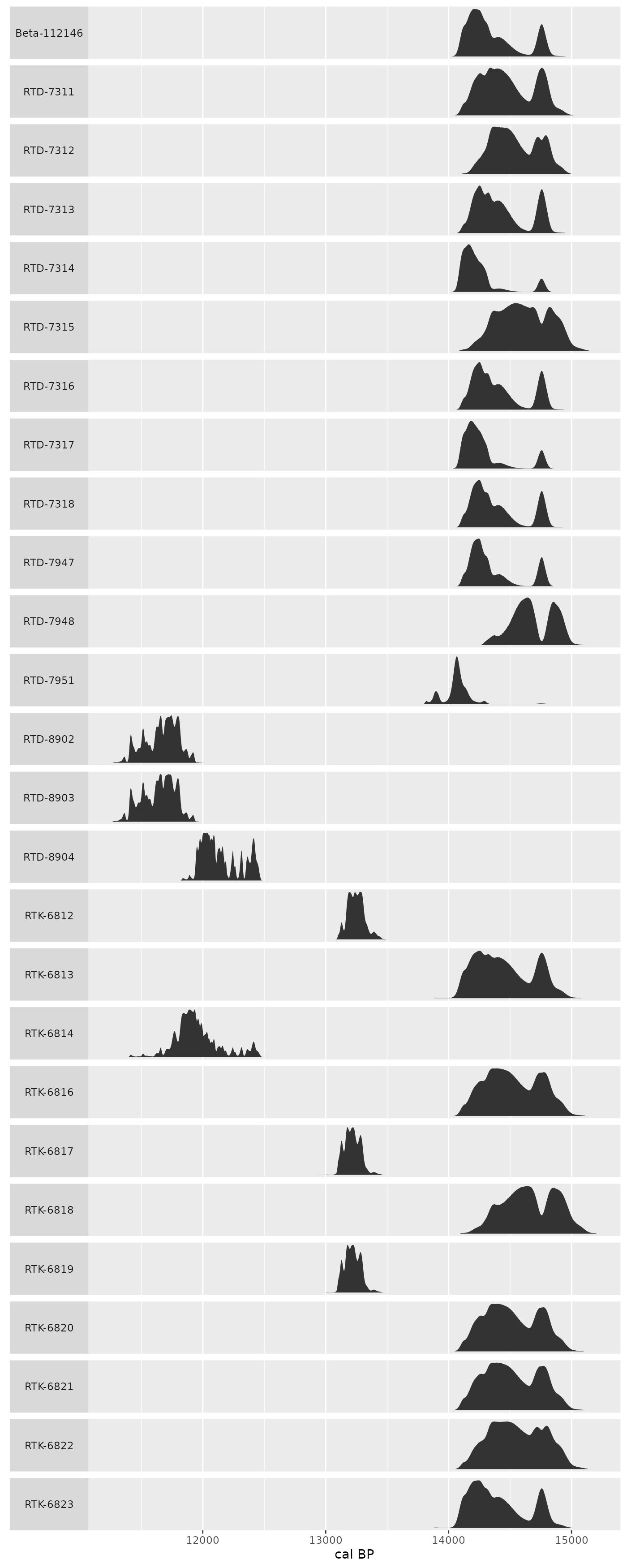

Modelling radiocarbon data

Summed probability distributions

In dplyr’s grammar, summing radiocarbon dates is a summary of the original data, because it reduces the number of observations. c14_sum is a wrapper for rcarbon::spd() that can be used in a dplyr statement.

shub1_radiocarbon %>% 
  group_by(phase) %>% 
  summarise(spd = c14_sum(cal, verbose = FALSE), .groups = "drop_last") ->
  shub1_spd
#> Warning: There were 34 warnings in `summarise()`.
#> The first warning was:
#> ℹ In argument: `spd = c14_sum(cal, verbose = FALSE)`.
#> ℹ In group 1: `phase = "Phase 1"`.
#> Caused by warning:
#> ! stratigraphr::c14_sum() is deprecated. Please use c14::c14_sum() instead.
#> ℹ Run `dplyr::last_dplyr_warnings()` to see the 33 remaining warnings.

head(shub1_spd)
#> # A tibble: 6 × 2
#>   phase   spd                   
#>   <chr>   <list>                
#> 1 Phase 1 <CalGrid [11,652 × 2]>
#> 2 Phase 2 <CalGrid [560 × 2]>   
#> 3 Phase 3 <CalGrid [473 × 2]>   
#> 4 Phase 4 <CalGrid [1,230 × 2]> 
#> 5 Phase 5 <CalGrid [1,324 × 2]> 
#> 6 Phase 6 <CalGrid [1,123 × 2]>

Bayesian calibration

See vignette("cql").

References

Millard, Andrew R. 2014. “Conventions for Reporting Radiocarbon Determinations.” Radiocarbon 56 (2): 555–59. https://doi.org/10.2458/56.17455.

Richter, Tobias, Amaia Arranz-Otaegui, Lisa Yeomans, and Elisabetta Boaretto. 2017. “High Resolution AMS Dates from Shubayqa 1, Northeast Jordan Reveal Complex Origins of Late Epipalaeolithic Natufian in the Levant.” Scientific Reports 7 (1): 17025. https://doi.org/10.1038/s41598-017-17096-5.

Wickham, Hadley. 2014. “Tidy Data.” Journal of Statistical Software 59 (10): 1–23. https://doi.org/10.18637/jss.v059.i10.